Predictive analytics empowers organizations to forecast future events by leveraging past data. When diving into this work, especially from a Minimum Viable Product (MVP) perspective, a streamlined yet robust tool is essential, and I love getting started with Scikit-Learn. It’s my initial playground for predictive analytics exploration.

Overview of Predictive Analytics

In a recent workshop - "Identifying Opportunities to Leverage AI Within the Manufacturing Sector", we explored the ability of AI to transform the manufacturing domain. Though the discussion primarily focused on manufacturing, the insights are applicable across many sectors.

At its core, predictive analytics is a domain-agnostic tool that is helpful across all domains, from healthcare to finance to retail and beyond.

The essence of predictive analytics lies in using historical data coupled with AI and machine learning to predict future outcomes. This foresight facilitates strategic decision-making, minimizes risks, and reduces downtime costs by flagging potential blockers and issues. This lets us optimize operations and maximize profits.

Some example applications:

• Manufacturing: Employing predictive maintenance to reduce machinery downtime.
• Healthcare: Augmenting early diagnosis and risk evaluation of diseases.
• FinTech: Strengthening fraud detection and credit risk assessment.

One bonus of predictive analytics lies in its transferability; we can borrow strategies from one domain to bring innovation to another.

From Problem to MVP Deployment

Transitioning from a problem statement to an MVP includes:

1. Problem outline to actionable insights.
2. Acquisition, cleaning, transformation, and structuring of data.
3. Model building and validation.
4. Fine-tuning models to align with the context.

I believe in people, process, and product forming the foundation of technical innovation. We can build great solutions by always starting with a question and a thorough understanding of the context, user narratives, and stakeholders.

Scikit-Learn: The MVP

While numerous tools and platforms are available for predictive analytics, Scikit-Learn stands out for its simplicity, ease of use, and efficiency, making it my preferred choice for MVPs and proof-of-concept projects. It’s a library that lowers the entry barrier, making the initial step into predictive modelling less daunting and more structured.

The benefit of Scikit-Learn lies in its gentle learning curve, which is helpful for individuals with a foundational understanding of Python. It has a well-organized, consistent, and intuitive API that accelerates onboarding. Furthermore, it has a rich library of algorithms for various machine learning tasks, providing a robust platform to build, experiment, and iterate on predictive models. The modular design promotes extensibility and interoperability with other libraries, enhancing its appeal for MVP development. The simple yet powerful nature of Scikit-Learn makes it an excellent choice for rapid prototyping, accelerating the process from concept to a working model, ready for real-world validation.

Problem Dimensions

Predictive analytics typically revolves around classification (categorizing data) or regression (forecasting continuous values):

• Classification: Categorizing data when the outcome variable belongs to a predefined set (e.g., 'Yes' or 'No').
• Regression: Forecasting continuous values when the outcome variable is real or continuous (e.g., weight or price).

Practical Example: Diabetes Progression Analysis

Let’s illustrate this with a practical example using a healthcare dataset on diabetes progression. Thanks to Scikit-Learn, accessing a toy diabetes dataset is simple. This dataset contains ten variables like age, BMI, and blood serum measurements for over 400 diabetes patients.

We’re looking to answer the following user stories:

• Healthcare Executive: Streamlining patient intake for timely intervention.
• Doctor: Identifying factors contributing to accurate diabetes progression prediction.
• Patient: Utilizing health metrics to understand and potentially mitigate diabetes progression risks.

import pandas as pd
from sklearn import datasets

# Load the diabetes dataset
diabetes = datasets.load_diabetes()
data = pd.DataFrame(data=diabetes.data, columns=diabetes.feature_names)
data["target"] = diabetes.target

Preliminary Analysis and Model Building

Before diving into model building, conducting an exploratory analysis is crucial. It often unveils insights that drive the choice of predictive models and features.

import matplotlib.pyplot as plt
import seaborn as sns

# Display the first few rows of the dataset
data.head()

# Summary statistics
data.describe()

# Correlation matrix
plt.figure(figsize=(10, 8))
sns.heatmap(data.corr(), annot=True)
plt.show()

The correlation matrix displays the relationships between various features and the target variable in the diabetes dataset. Here are the key insights from the correlation matrix:

BMI and Target Correlation:

• There's a positive correlation between BMI (Body Mass Index) and the target variable, suggesting that as BMI increases, the diabetes measure also tends to increase.

Blood Pressure (bp) and Target Correlation:

• Blood pressure shows a positive correlation with the target variable. This indicates that higher blood pressure values are associated with higher diabetes measures.

Negative Correlation of S3 and Target:

• S3 exhibits a negative correlation with the target variable, indicating that higher values of S3 are associated with lower values of the diabetes measure.

Correlation Among Features:

• The features S1 and S2 show a high positive correlation, indicating a strong linear relationship between them.
• S4 and S3 have a strong negative correlation, showing that as one variable increases, the other tends to decrease significantly.
• The S4 and S2 and S4 and S5 pairs also exhibit strong positive correlations, suggesting that these features are likely moving together.

Age Correlation:

• Age has a positive correlation with various features, including blood pressure (bp), S5, and S6, and a lesser but still significant positive correlation with the target variable.

Data Preprocessing

Data Preprocessing is vital in building a machine learning model as it prepares the raw data to be fed into the model, ensuring better performance and more accurate predictions. In this process, standardizing the data and splitting it into training and testing sets are essential steps.

The first objective here is to have separate datasets for training and evaluating the model. A common rule of thumb is the 80-20 rule, where 80% of the data is used for training and the remaining 20% for testing. This ratio provides a good balance, ensuring that the model has enough data to learn from while still having a substantial amount of unseen data for evaluation.

Second, standardization is crucial for many machine learning algorithms, especially distance-based and gradient descent-based algorithms. It scales the data to have a mean of 0 and a standard deviation of 1, thus ensuring that all features contribute equally to the computation of distances or gradients.

from sklearn.model_selection import train_test_split
from sklearn.preprocessing import StandardScaler

# Splitting the data into training and testing sets
X = data.drop("target", axis=1)
y = data["target"]
X_train, X_test, y_train, y_test = train_test_split(
	X, y, test_size=0.2, random_state=42
)

# Standardize the data
scaler = StandardScaler()
X_train = scaler.fit_transform(X_train)
X_test = scaler.transform(X_test)

Model Building - Linear Regression

Linear Regression is a simple first step in predictive analytics due to its straightforwardness and ease of interpretation. It operates under supervised learning, establishing a linear relationship between the input features and the target variable.

from sklearn.linear_model import LinearRegression

# Create and train the model
lr = LinearRegression()
lr.fit(X_train, y_train)

The simplicity of Linear Regression lies in both its single-line training command and its model output, which is easy to interpret. The coefficients tell us the weight or importance of each feature, while the intercept gives us a baseline prediction when all feature values are zero. This interpretability makes Linear Regression an excellent starting point for model building and a valuable tool for communicating findings to stakeholders.

Evaluating and Visualizing Outcomes

Evaluating a model's performance lies in understanding its accuracy and identifying areas of improvement. One standard metric used in regression tasks is the Mean Squared Error (MSE), which quantifies the average squared difference between actual and predicted values. A lower MSE value indicates a better fit of the model to the data, although it's important to note that MSE is sensitive to outliers.

Visualizing the relationship between actual and predicted values further illuminates the model's performance. A scatter plot is a handy tool for this purpose, clearly representing how well our model's predictions align with the actual values. The closer the points cluster around the line of identity (a line with a slope of 1, passing through the origin), the better our model makes accurate predictions.

from sklearn.metrics import mean_squared_error
import numpy as np

# Predictions
y_pred = lr.predict(X_test)

# Calculating and displaying the Mean Squared Error
mse = mean_squared_error(y_test, y_pred)
print(f"Mean Squared Error: {mse}")

# Visualizing the actual values and predicted values
plt.scatter(
	y_test, y_pred, alpha=0.5
)  # Added alpha for better visualization if points overlap
plt.xlabel("Actual values")
plt.ylabel("Predicted values")
plt.title("Actual values vs Predicted values")

# Adding line of identity
lims = [
	np.min([plt.xlim(), plt.ylim()]),  # min of both axes
	np.max([plt.xlim(), plt.ylim()]),
]  # max of both axes

# now plot both limits against each other
plt.plot(lims, lims, color="red", linestyle="--")
plt.xlim(lims)
plt.ylim(lims)

plt.show()

In this visualization, the red dashed line represents the line of identity, where a perfect model would have all points lie. Deviations from this line indicate prediction errors. Such a visual aid provides a qualitative insight into the model's performance. It serves as a tangible explanation tool for stakeholders, showcasing the model's strengths and areas needing enhancement in a digestible format.

Transitioning to a Classification Problem

Our first approach used a linear regression model to predict the continuous target variable representing diabetes progression. However, as evaluated by the Mean Squared Error, the model's performance has room for improvement.

Transforming the problem into a binary classification scenario often brings a different perspective and could lead to better performance. In some instances, by changing it into a binary classification problem, we aim to predict whether a patient's diabetes has progressed based on a predetermined threshold.

Let's define progression as a binary variable: `1` if the progression measure is above a certain threshold and `0` otherwise. We'll choose the median of the target variable in the training set as the threshold for simplicity:

python
from sklearn.preprocessing import Binarizer

# Defining the threshold
threshold = np.median(y_train)

# Transforming the target variable
binarizer = Binarizer(threshold=threshold)
y_train_class = binarizer.transform(y_train.values.reshape(-1, 1))
y_test_class = binarizer.transform(y_test.values.reshape(-1, 1))

We can proceed with a classification model now that we have our binary target variable. A common choice for such problems is Logistic Regression:

from sklearn.linear_model import LogisticRegression

# Training the Logistic Regression model
lr_class = LogisticRegression()
lr_class.fit(X_train, y_train_class.ravel())

# Making predictions on the test set
y_pred_class = lr_class.predict(X_test)

Evaluate the Model

After training, evaluating the model on unseen data is essential to gauge its performance and robustness. Scikit-Learn provides various tools, including a classification report and a confusion matrix, which are used for classification problems. Through these metrics, we can understand the model's accuracy, misclassification rate, and other crucial performance indicators.

Classification Report

The classification report provides the following key metrics for each class and their averages:

• Precision: The ratio of correctly predicted positive observations to the total predicted positives. High precision relates to the low false positive rate.
• Recall (Sensitivity): The ratio of correctly predicted positive observations to the total observations in the actual class. It tells us what proportion of the actual positive class was identified correctly.
• F1-Score: The weighted average of Precision and Recall.
• Support: The number of actual occurrences of the class in the specified dataset.

from sklearn.metrics import classification_report

# Evaluating the model
class_report = classification_report(y_test_class, y_pred_class)
print(class_report)

            precision    recall  f1-score   support

         0.0       0.77      0.82      0.79        49
         1.0       0.76      0.70      0.73        40

    accuracy                           0.76        89
   macro avg       0.76      0.76      0.76        89
weighted avg       0.76      0.76      0.76        89

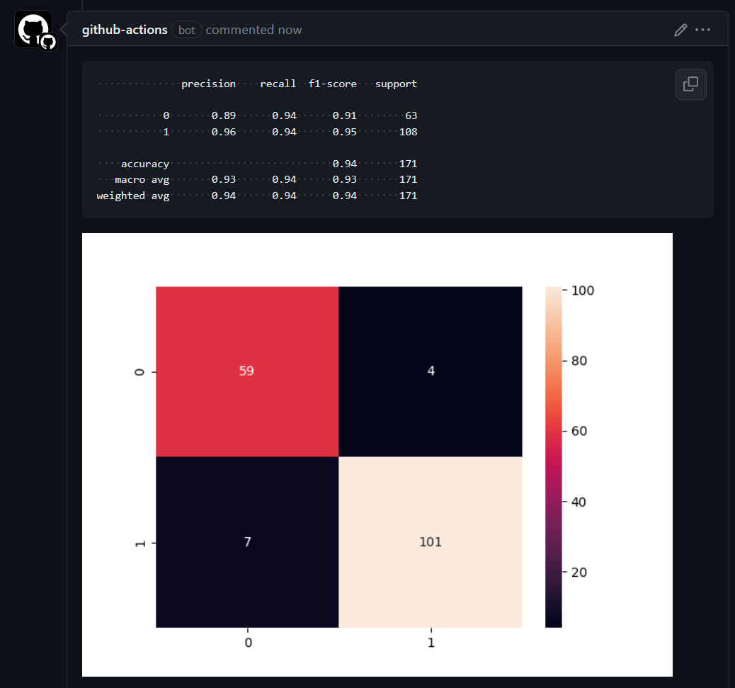
Confusion Matrix

A Confusion Matrix is a table used to evaluate a classification model's performance. It not only gives insight into the errors made by a classifier but also the types of errors being made.

from sklearn.metrics import ConfusionMatrixDisplay

disp = ConfusionMatrixDisplay.from_estimator(
	lr_class,
	X_test,
	y_test_class,
	display_labels=["Not Progressed", "Progressed"],
	cmap=plt.cm.Blues,
)
plt.show()

In this visualization, each matrix column represents the instances in a predicted class, while each row represents the instances in an actual class. The label “Not Progressed” is mapped to 0, and “Progressed” is mapped to 1. The diagonal elements represent the number of points for which the predicted label is equal to the true label, while off-diagonal elements are those that the model misclassifies.

This colour-coded matrix represents the classifier's performance, where darker shades represent higher values. Hence, the diagonal would be distinctly darker for a well-performing model than the rest of the matrix.

Dimensionality Reduction and Visualization

In Predictive Analytics, our models often work with many dimensions, each representing a different data feature. However, navigating through high-dimensional space is tricky and not intuitive. This is where dimensionality reduction techniques like t-SNE (t-Distributed Stochastic Neighbor Embedding) come into play, acting as a bridge from the high-dimensional to a visual, often 2-dimensional, representation.

Visualizing high-dimensional data in a lower-dimensional space, like 2D, helps understand the data distribution and the model's decision boundaries.

from sklearn.manifold import TSNE

# Create a TSNE instance
tsne = TSNE(n_components=2, random_state=42)

# Fit and transform the data
transformed_data = tsne.fit_transform(X_test)

# Visualizing the 2D projection with color-coding
plt.scatter(
	transformed_data[:, 0],
	transformed_data[:, 1],
	c=np.squeeze(y_test_class),
	cmap="viridis",
	alpha=0.7,
)
plt.xlabel("Dimension 1")
plt.ylabel("Dimension 2")
plt.title("2D TSNE")
plt.colorbar(label="Progressed (1) vs Not Progressed (0)")
plt.show()

The colour-coded scatter plot produced in the code above shows how the diabetes progression (categorized as Progressed and Not Progressed) is distributed across two dimensions. Each point represents a patient, and the colour indicates the progression status. This visual can reveal clusters of similar data points, outliers, or patterns that might correlate with the predictive model's performance.

This 2D visualization might unveil hidden relations between features and the target variable or among the features themselves. Such insights can guide further feature engineering, model selection, or hyperparameter tuning to enhance the model's predictive power potentially.

Such visualizations can also be a powerful communication tool when discussing the model and the data with non-technical stakeholders. It encapsulates complex, high-dimensional relationships into a simple, interpretable form, making the conversation around the model's decisions more accessible.

Recap

This walkthrough demonstrates how to quickly move from a real-world problem to a simple MVP using Scikit-Learn for predictive analytics. The journey from understanding the problem, preprocessing the data, building, and evaluating the models, to finally visualizing the outcomes is filled with learning at every step. With simple but powerful tools like Scikit-Learn, predictive analytics is accessible for all stakeholders.